Qdrant + Embeddings + LLM + Orchestration: The RAG Stack That Keeps Your AI Grounded
Qdrant + Embeddings + LLM + Orchestration: The RAG Stack That Keeps Your AI Grounded
One-line verdict: This four-layer stack — index documents in Qdrant, encode meaning with an embedding model, retrieve by semantic similarity, generate with an LLM — solves hallucination at the source: your AI answers from documents you control, not from a model’s best guess at what it absorbed during training.
This post is about the full retrieval pipeline. The focus is on how all four layers fit together in production — collections, payloads, filtered search, and the orchestration code that ties them into a working RAG system. If you want to go deeper on vector search mechanics specifically (HNSW index structure, distance metrics, approximate vs. exact recall trade-offs), that’s a separate thread. This post picks up at the practical question most people hit first: how do I stop my chatbot from making things up?
The Problem This Stack Solves
Every LLM has a knowledge cutoff and a hallucination problem. It was trained on a snapshot of the internet, it doesn’t know about your private documents or recent events, and when it doesn’t know something it will often generate plausible-sounding text anyway rather than admit the gap.
The standard fix — stuffing more context into the system prompt — stops scaling fast. At some point the prompt is too long, the latency climbs, the cost multiplies, and the model’s attention gets diluted across thousands of tokens of background that’s mostly irrelevant to the current question.
RAG fixes this properly. Instead of pre-loading everything, you retrieve only the relevant pieces at query time. The model gets a tight, relevant context window and produces grounded, attributable answers. The retrieval layer is the hard part, and Qdrant is where that retrieval lives.
I’ve been running this stack in production for several months. The setup took a few hours. The operational overhead is close to zero. This is the guide I wish I’d had.
The Processing Flow: Four Layers, Two Phases
[Ingestion]
Documents → Chunker → Embedding Model → Qdrant (upsert)

[Query]
User Question → Embedding Model → Qdrant (query_points) → Top-K Chunks → LLM → Grounded Answer
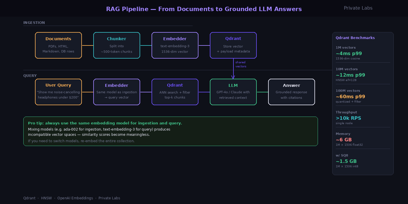
The pipeline splits cleanly into two phases. Ingestion runs once (and again when documents change): you chunk your documents, embed each chunk, and upsert the vectors and their metadata into Qdrant. The query phase runs on every user request: embed the question, search Qdrant for the closest vectors, pull the text from those payloads, and hand everything to the LLM.
Each layer is a prerequisite for the next. None is optional.
Why Each Layer Is Non-Negotiable
Qdrant: The Retrieval Engine
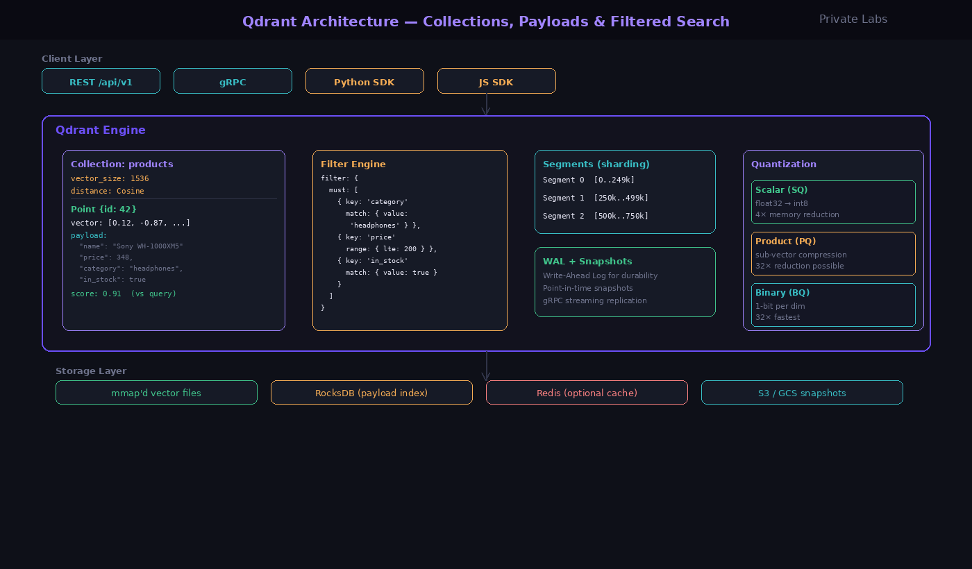
Qdrant stores high-dimensional float vectors alongside JSON metadata called payloads. When a query vector arrives, it traverses an HNSW (Hierarchical Navigable Small World) index to find the geometrically nearest stored vectors — the documents semantically closest to the question — in milliseconds, even across millions of points.
The critical configuration decision happens at collection creation and cannot be changed afterwards: the vector size (must exactly match your embedding model’s output dimensions) and the distance metric (Cosine for text, almost always).
from qdrant_client import QdrantClient
from qdrant_client.models import Distance, VectorParams

client = QdrantClient(url="http://localhost:6333")

client.create_collection(
    collection_name="knowledge_base",
    vectors_config=VectorParams(
        size=1536,                # must match your embedding model exactly
        distance=Distance.COSINE,
    ),
)
Payloads are what make Qdrant genuinely useful versus a bare vector index. Every point carries a JSON object alongside its vector — the original text, the source URL, a timestamp, a category, anything you want. Payload filters apply inside the HNSW traversal, not after retrieval, so filtering 90% of a collection by metadata doesn’t cost 90% more query time.
from qdrant_client.models import PointStruct

client.upsert(
    collection_name="knowledge_base",
    wait=True,
    points=[
        PointStruct(
            id=1,
            vector=[0.05, 0.61, 0.76, 0.74],
            payload={
                "text": "Berlin is the capital of Germany",
                "source": "geography-basics.md",
                "verified": True,
            }
        ),
        PointStruct(
            id=2,
            vector=[0.19, 0.81, 0.75, 0.11],
            payload={
                "text": "London is in the UK",
                "source": "geography-basics.md",
                "verified": True,
            }
        ),
    ],
)
wait=True blocks until the server confirms the write is complete and indexed. Running queries against data that hasn’t finished indexing is a silent failure mode that costs hours to diagnose.
What Qdrant provides: Semantic retrieval at low-millisecond latency over millions of documents, with payload-filtered search that doesn’t degrade performance.
Embedding Model: The Semantic Bridge
An embedding model converts text into a dense float vector. Semantically similar sentences end up geometrically close in that vector space. This is the mechanism that makes “what is the capital of Germany?” retrieve “Berlin is the capital of Germany” even though there’s no keyword overlap.
The single most important rule: use the same embedding model for ingestion and queries, always. Different models produce incompatible vector spaces. If you indexed with text-embedding-3-small and query with text-embedding-3-large, the similarity scores become meaningless — high scores no longer indicate relevant content. When upgrading embedding models, re-embed the entire collection from scratch.
The size in your Qdrant collection must match the model’s output dimensions. For OpenAI text-embedding-3-small, that’s 1536 dimensions.
# Pseudocode — replace embed() with your actual embedding function
def embed(text: str) -> list[float]:
    # Returns a list of floats with length == your collection's size parameter
    ...

# Same function called in both phases:
ingestion_vector = embed(document_chunk)   # at indexing time
query_vector = embed(user_question)        # at query time
What the embedding model provides: A shared coordinate system where meaning, not keywords, determines proximity.
LLM: The Answer Generator
The LLM is the last layer, not the first. Its job is not to know things — it’s to synthesize and articulate, given a context window you’ve filled with relevant, verified content from Qdrant.
This is the architectural shift that eliminates hallucination. The model isn’t being asked to remember anything. It’s being asked to read the documents you retrieved and answer based on them. When the retrieval is good, the answers are grounded. When it cites something wrong, the bug is in the retrieval layer, not the model — which means it’s debuggable.
# After retrieval from Qdrant:
hits = client.query_points(
    collection_name="knowledge_base",
    query=query_vector,
    limit=5,
    with_payload=True,
).points

# Build context from retrieved payloads
context = "\n\n".join(hit.payload["text"] for hit in hits)

# Ground the LLM in retrieved content
answer = llm.generate(
    f"Answer based only on the following context:\n\n{context}\n\nQuestion: {user_query}"
)
The instruction “answer based only on the following context” is load-bearing. Without it, the model will blend retrieved content with its own training data — which is exactly the hallucination problem you’re trying to eliminate.
What the LLM provides: Fluent synthesis of retrieved content into a coherent, contextual answer.
Orchestration: The Glue That Makes It a System
Qdrant, an embedding model, and an LLM are three separate services. Orchestration is the code that connects them into a reliable pipeline: calling the right service in the right order, handling failures, managing batch sizes during ingestion, and applying filters that scope retrieval to the right subset of data.
The orchestration layer is also where multi-tenancy lives. If you’re serving multiple users from the same Qdrant collection, payload filters enforce isolation:
from qdrant_client.models import Filter, FieldCondition, MatchValue

# Scope search to this user's documents only
user_filter = Filter(
    must=[
        FieldCondition(key="user_id", match=MatchValue(value=current_user_id)),
    ]
)

hits = client.query_points(
    collection_name="knowledge_base",
    query=query_vector,
    query_filter=user_filter,   # applied during HNSW traversal, not after
    limit=5,
    with_payload=True,
).points
The filter runs inside the HNSW search rather than post-retrieval. That’s the difference between a proper multi-tenant RAG system and one that leaks data between users.
What orchestration provides: A reliable, debuggable control plane that connects retrieval, embedding, and generation into a single coherent system.
How Search Actually Works
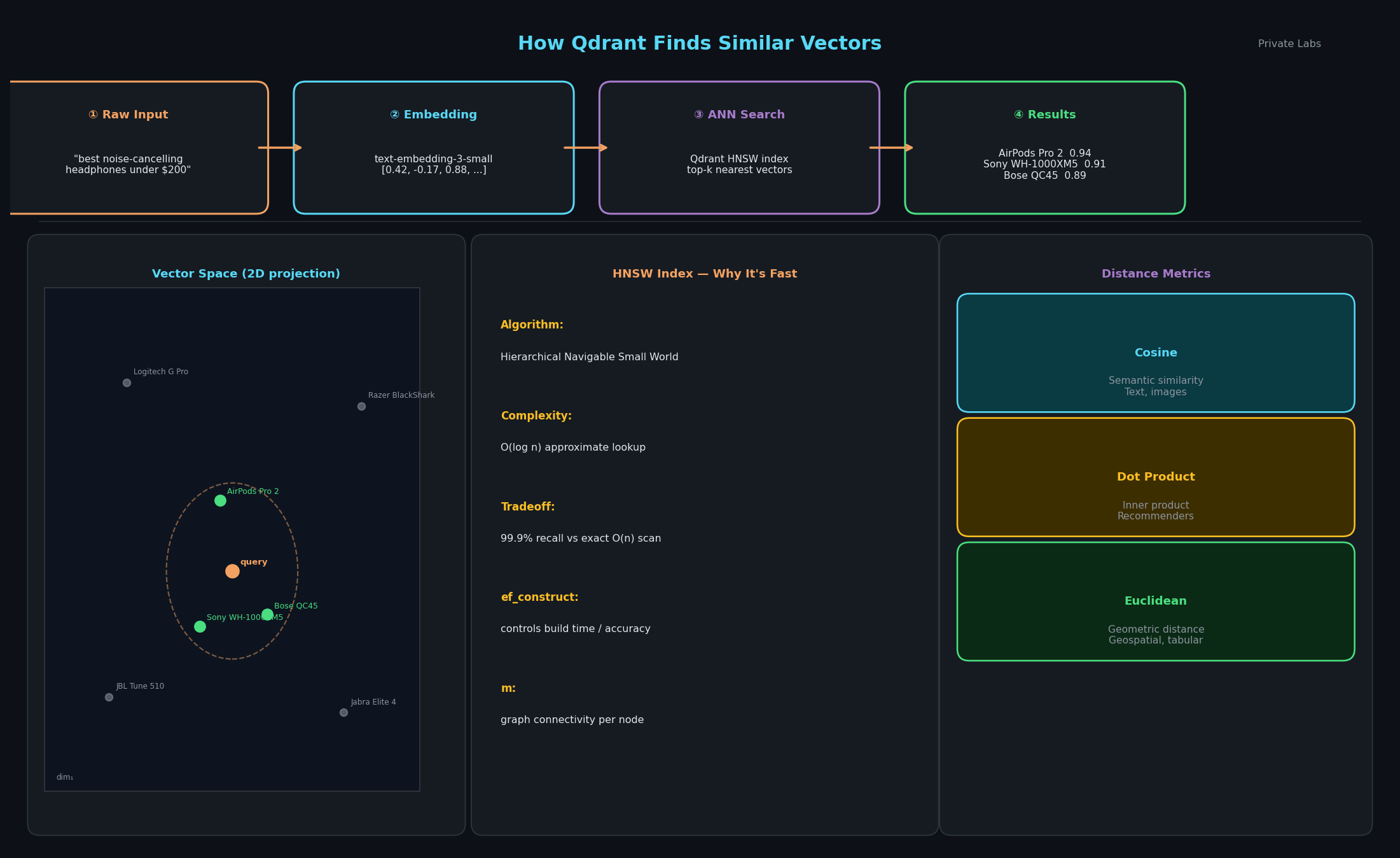
The current recommended API is query_points(). The older search() method still works in qdrant-client 1.18.0 but new code should use query_points.
from qdrant_client.models import Filter, FieldCondition, MatchValue, SearchParams

results = client.query_points(
    collection_name="knowledge_base",
    query=[0.2, 0.1, 0.9, 0.7],          # query vector — same dimensions as collection
    query_filter=Filter(
        must=[
            FieldCondition(key="verified", match=MatchValue(value=True))
        ]
    ),
    search_params=SearchParams(hnsw_ef=128, exact=False),
    limit=5,
    with_payload=True,
).points

for point in results:
    print(point.id, point.score, point.payload)
    # point.score: 0–1, higher = more similar to query
SearchParams(hnsw_ef=128) controls how deeply the HNSW graph is explored. Higher values improve recall at the cost of latency. The right value is workload-dependent — start at 64 and tune from there. exact=True bypasses HNSW entirely for a brute-force scan: useful for debugging small collections, expensive at scale.
Each returned ScoredPoint has .id, .score, and .payload. The score is the similarity measure — with Cosine distance, 1.0 is identical, 0.0 is orthogonal.
Real usage note: I spent two hours debugging a RAG pipeline where retrieval quality was consistently poor. The bug turned out to be hnsw_ef set to 16 (the default) on a collection with aggressive filtering — low ef plus heavy filtering meant the HNSW search was terminating before finding enough candidates. Bumping to 64 fixed recall immediately. Check hnsw_ef early when filtered search is underperforming.
The Compounding Effect: When Retrieval Gets Better Over Time
Run this stack for six months and three things compound simultaneously.
First, your data quality improves. Chunking strategy determines retrieval quality more than any other variable. After a few months of running this in production, you’ll have accumulated real evidence of which chunks surface for which queries, which filters eliminate false positives, and where the embedding model loses coherence. Each tuning iteration compounds into better retrieval — and better retrieval means better LLM answers without any model upgrade.
Second, payload metadata becomes a precision instrument. Early on, I stored only text and source in payloads. After a few months, I’d added section_type, date_indexed, confidence_score, and product_category — all filterable, all making retrieval more precise. Each new payload field is a new dimension of control over what the LLM sees.
Third, the diagnostic loop shortens. When a RAG answer is wrong, the question is always “was it retrieval or generation?” With Qdrant’s payload-rich results, you can inspect exactly which chunks were retrieved, score them by relevance, and determine whether the failure was a retrieval miss or a synthesis error. After months of this, you develop fast intuition about where bugs live and how to fix them. The system becomes easier to maintain as it becomes more mature.
Why This Stack Gets More Valuable Over Time
Three forces are pushing in the same direction.
Embedding models will keep improving. New embedding models regularly push the boundary of what semantic similarity can capture — longer context, better cross-lingual transfer, domain-specific fine-tunes. Because Qdrant is model-agnostic, you can upgrade your embedding model by recreating the collection and re-running ingestion. The retrieval infrastructure doesn’t change; only the quality of the coordinate system does.
Payload filtering will become the primary differentiation. As RAG becomes standard infrastructure, the competitive edge shifts to retrieval precision. Who surfaces the right document, not just a related one. Payload-filtered semantic search — scoped by date, category, confidence, user, source quality — is where that precision lives. Qdrant’s filter architecture (applied during index traversal, not post-retrieval) makes this practical at production scale.
Multi-modal retrieval will extend this same pattern. Text embeddings today, image embeddings tomorrow, code embeddings already. Qdrant handles any fixed-dimension float vector with the same API. The retrieval pattern — embed, index, search, generate — applies across modalities. The stack you build for text RAG today is the foundation for multi-modal RAG when the use case requires it.
Practical Setup
Everything below assumes a local Docker-based Qdrant server and qdrant-client 1.18.0.
1. Start Qdrant:
docker run -p 6333:6333 -p 6334:6334 \
    -v "$(pwd)/qdrant_storage:/qdrant/storage:z" \
    qdrant/qdrant
2. Install the client:
pip install qdrant-client
# include FastEmbed for local embedding inference:
pip install "qdrant-client[fastembed]"
3. Full ingestion + query pipeline:
from qdrant_client import QdrantClient
from qdrant_client.models import Distance, VectorParams, PointStruct

client = QdrantClient(url="http://localhost:6333")

# ── Ingestion (run once, or on document updates) ────────────────────────────

client.create_collection(
    "knowledge_base",
    vectors_config=VectorParams(size=1536, distance=Distance.COSINE)
)

# embed() = your embedding model call; doc_chunks = list of (text, source_url)
client.upsert(
    "knowledge_base",
    points=[
        PointStruct(
            id=i,
            vector=embed(chunk),
            payload={"text": chunk, "source": source_url}
        )
        for i, (chunk, source_url) in enumerate(doc_chunks)
    ]
)

# ── Query (runs on every user request) ─────────────────────────────────────

query_vector = embed(user_query)

hits = client.query_points(
    collection_name="knowledge_base",
    query=query_vector,
    limit=5,
    with_payload=True,
).points

context = "\n\n".join(hit.payload["text"] for hit in hits)
answer = llm.generate(f"Context:\n{context}\n\nQuestion: {user_query}")
4. For unit tests — no Docker required:
# In-memory client: full API, no server, zero setup
client = QdrantClient(":memory:")
5. Checklist before going to production:
wait=Trueon all upserts in ingestion pipelines- Same embedding model in ingestion and query — enforce this in config, not by convention
textstored in every payload — avoid secondary lookups at query timeuser_idororg_idin payloads if multi-tenant — filter on every queryhnsw_eftuned for your filter selectivity — start at 64, measure recall
The Bottom Line
Without RAG, an LLM answers from training data — fixed in time, oblivious to your private documents, and confident when it shouldn’t be.
The shift this stack makes:
Before: User question → LLM → answer from training data (may hallucinate)
After:  User question → embed → Qdrant → retrieved chunks → LLM → grounded answer
The added complexity is a Docker container, one Python library, and an orchestration loop that fits in under fifty lines. What you get in return: an AI that answers from documents you control, whose failures are debuggable, and whose quality improves as your data and tuning improve.
If you’re building anything with LLMs that needs to be accurate — a support bot, an internal knowledge assistant, a document Q&A system — the retrieval layer isn’t optional. It’s the thing that makes the difference between a demo and a production system.
This stack makes that layer practical to build and maintain.
Have questions about chunking strategy, multi-tenant isolation patterns, or embedding model selection for a specific domain? Drop a comment. Those are the parts where the implementation details matter most, and I’m happy to go deeper on any of them.